Technical2026-10-25
Variable-speed irrigation pumps should follow a verified hydraulic demand map, not one pressure setpoint copied across every zone. A variable frequency drive (VFD) changes motor and pump speed so one centrifugal pump can serve changing flows, but the acceptable speed range is bounded by the pump curve, static head, required field pressure, source conditions, motor cooling, drive current and minimum stable flow. Build those boundaries first, then tune control inside them.
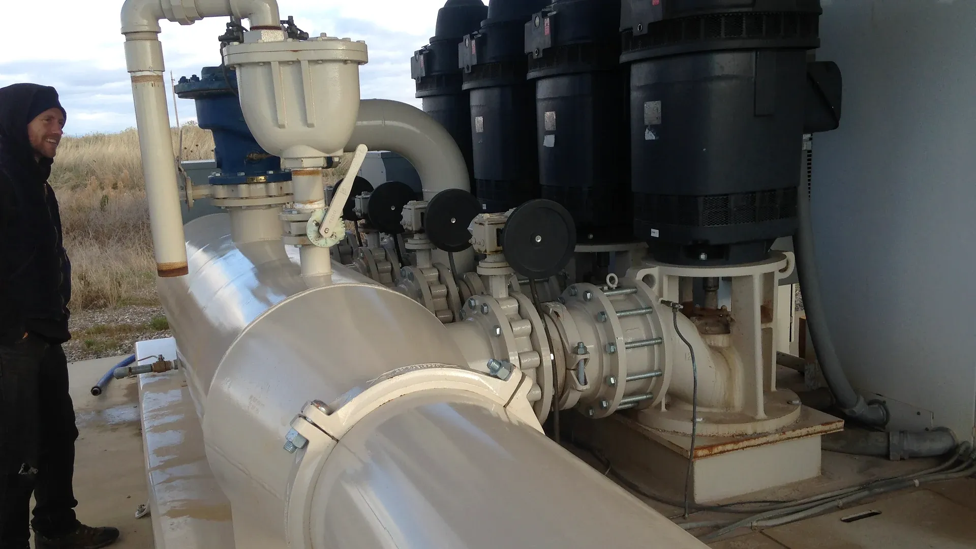
A real automated canal pumping station for pressurized farm irrigation, with multiple pumps, manifold pipework and control connections visible. The photograph documents agricultural irrigation equipment; it does not prove that a particular speed or pressure setting is suitable.
This guide gives a field method for matching VFD pump speed to small and large irrigation zones. It uses affinity laws as an initial calculation, then requires measured operating points and equipment-specific limits. Electrical design, programming and energized testing belong to qualified personnel following the pump, motor and drive instructions.
List every permitted zone combination rather than writing “variable flow” in the specification. For each job, record the open valves, design flow, minimum pressure at the defined delivery node, elevation, filtration state, emitter or sprinkler operating range and source-water level. Include normal combinations, the smallest legitimate zone, peak demand and approved flushing duties. Exclude combinations the piping or water right does not permit.
Rather than relying on mechanical throttling valves that waste hydraulic energy, modern variable frequency drives modulate brushless centrifugal water pumps to track changing zone flow requirements directly.
The irrigation pump flow and total dynamic head method establishes the full-speed duty. This article extends that work across changing demand. If the required head was guessed from the pump nameplate or a static gauge reading, changing speed cannot repair the missing hydraulic design.
| Operating job | Required flow | Required delivery pressure | Source and field condition to record | Control implication |
|---|---|---|---|---|
| Small drip block | Lowest legitimate steady demand | Pressure needed after filtration and regulation | Minimum source lift and clean/dirty filter states | May establish minimum useful pump speed |
| Two drip blocks | Sum of simultaneous emitter demand | Worst hydraulic path | Valve combination and elevation | Pressure loop should move smoothly to a new duty |
| Sprinkler set | Nozzle demand plus approved allowances | Pressure at the defined sprinkler node | Wind is logged but is not a pump-control input by itself | May require a different verified setpoint |
| Peak combination | Largest allowed demand | Critical remote-node pressure | Lowest seasonal source level | Tests maximum speed, motor current and suction margin |
| Flush operation | Specified cleaning flow | Enough head to sustain required velocity | Discharge route and duration | Separate supervised mode may be necessary |
A VFD continuously changes electrical frequency and voltage so an appropriate motor can operate over a controlled speed range. Soft starting is only one possible function. A soft starter reduces starting stress but normally hands the motor to fixed line frequency after acceleration. A control valve can reduce downstream pressure at fixed pump speed, but the pump still develops the operating point created by the pump and system curves.
Choose the control method from the duty. If one pump serves a nearly constant flow and head, a VFD may add cost, heat and maintenance without meaningful operating benefit. If zone flow, lift or pressure changes materially, speed control may avoid persistent throttling and can keep delivery closer to the field requirement. Do not describe every VFD installation as an energy project; first quantify the hours and loads at each job.
For the same centrifugal pump and impeller, over an appropriate speed range, the common screening relationships are Q₂/Q₁ = N₂/N₁, H₂/H₁ = (N₂/N₁)² and P₂/P₁ ≈ (N₂/N₁)³. Flow Q changes approximately with speed N, head H with speed squared, and shaft power P with speed cubed. These relationships move the pump curve; they do not determine where it intersects the actual system curve.
For steep downhill zones where variable frequency drives cannot decelerate below minimum cooling speeds, downstream manifolds incorporate hydraulic pressure regulating valves to dissipate excess static elevation head.
The Utah State University Extension guide to variable frequency drives for irrigation pumps identifies varying flow or pressure as a key application and also calls for motor, amperage, environmental, cooling and power-quality checks. Use the actual pump curves and drive documentation for selection. The equations below are transparent estimates, not substitute performance data.
Suppose a tested point at 1,760 rpm is 120 m³/h at 50 m of head and 24 kW shaft power. At 85% speed, the affinity estimates are 102 m³/h, 36.1 m of head and 14.7 kW: 120 × 0.85, 50 × 0.85² and 24 × 0.85³. These values describe corresponding points on a scaled pump curve. They do not promise that the irrigation system will operate at exactly 102 m³/h or consume exactly 14.7 kW.
Now assume the route needs 18 m of static head before friction and field pressure are considered. Reducing speed does not reduce that elevation requirement. The system curve retains its static component, so actual flow can fall much faster than the simple 15% estimate or disappear when the reduced-speed pump curve cannot cross the required head. Plot the scaled pump curves against the system curve before accepting a low-speed job.
A system curve combines the head that does not depend on flow with losses that increase as flow rises. Static elevation, pressurized destination and some fixed boundary requirements remain even at low flow. Pipe, fitting, valve and filter losses change with flow and equipment state. One curve cannot represent a small uphill block, a large level block and a backwash route if their paths differ.
Use the pump operating-point guide for changing zones to plot each intersection. Mark the permitted pump envelope, best-efficiency region, maximum motor load, available suction margin and any manufacturer limits on continuous operation. A VFD does not make every point below the full-speed curve acceptable.
If one remote zone lacks pressure while nearby zones are over-pressurized, inspect the route, valves, filters and zoning. Raising the common pressure target may increase leakage and energy use without correcting an undersized branch or blocked component. The drip irrigation pressure-budget worksheet keeps each loss assigned to its real location.
Constant discharge pressure is common, but it is not automatically the best representation of crop delivery. A sensor at the pump protects and controls a different boundary from a sensor at a remote mainline node. A remote sensor can represent field demand more directly, but its communication, power, calibration and failure response become part of the control system.
Define the controlled variable, sensor range, uncertainty, sample interval, filtering, setpoint source and fallback. State what happens if the reading is frozen, implausible, missing or inconsistent with flow. Pressure, flow, valve status, source level, motor current and speed should be time-aligned so operators can distinguish demand changes from sensor or equipment faults.
| Control approach | Useful when | Main evidence | Common failure to prevent |
|---|---|---|---|
| Local discharge-pressure control | Downstream network is predictable | Pressure sensor plus zone-specific required head | Remote zone under-pressure hidden by a normal pump reading |
| Remote-node pressure control | Critical field node changes with demand | Reliable telemetry, local high-pressure protection and fallback | Runaway speed after loss of the remote signal |
| Flow or speed schedule by zone | Zone duties are stable and well tested | Confirmed valve state and commissioned setpoints | Wrong schedule after a field modification |
| Cascade pressure with limits | Pressure must adapt within a verified envelope | Pressure, flow, speed, current and protective limits | Integrator windup or hunting during valve transitions |
| Manual fixed-speed fallback | Temporary supervised recovery is designed | Approved jobs, speed ceiling and field pressure check | Fallback treated as unrestricted normal operation |
The drive’s lowest programmable frequency is not the pump system’s minimum operating speed. At low speed the pump may fail to overcome static head, a vertical motor may lose adequate cooling, a shaft or bearing may enter an undesirable range, check valves may become unstable, and the pump may operate below its required minimum flow. The water source and lubrication arrangement can add further limits.
Find the highest applicable lower bound: minimum speed from the pump supplier, motor cooling requirement, drive and cable limits, minimum continuous pump flow, minimum head needed for the smallest zone and stable sensor/control behaviour. If the smallest zone falls below that boundary, redesign the zone, use a correctly sized smaller pump, add purpose-designed storage or use an engineered bypass only if the complete system supports it. Do not waste water through an improvised bleed just to keep the drive running.
A generic “never below 30 Hz” or “always safe above 50% speed” rule ignores motor poles, base frequency, pump construction, static head and duty. Record the actual rpm when available rather than relying only on displayed hertz. Verify stable flow, pressure, current, vibration and temperature at the lowest approved job after the system reaches steady operation.
Collect motor nameplate voltage, phase, full-load amperes, service factor, base frequency, rated speed, insulation and enclosure. Confirm whether the existing motor is suitable for inverter operation and the intended speed range. Long motor leads, reflected-wave voltage, switching frequency, altitude, ambient heat and enclosure ventilation can change the required filters, reactors, cable and derating.
Size the drive by the applicable current and duty, not by matching one horsepower label. Confirm input supply, phase conversion if any, overload behaviour, short-circuit protection, disconnects, earthing, surge protection and harmonic obligations with qualified electrical parties. Keep dust, moisture, fertilizer vapour, rodents and direct solar heating out of the enclosure using a design suitable for the site.
After electrical work, verify rotation using the approved method before full hydraulic operation. Check shaft, coupling, gearbox, line-shaft, seal and bearing speed limits. A motor that tolerates lower frequency does not prove that every driven component or lubrication system does. Record any critical speed bands the supplier says to skip.
Define the sequence for opening a delivery path, starting the pump, building pressure, admitting another zone, removing a zone and stopping. Valve movement and pump speed response must not create deadhead, loss of prime, reverse flow or a damaging transient. The pump and valve interlock guide provides the related operating-permission framework.
Protective functions retain priority over the normal pressure loop. Examples can include source low level, loss of flow, high discharge pressure, low suction condition, motor overload, drive overtemperature and emergency stop where the design requires them. Setpoints and delays must come from the actual equipment and process; they are not universal values to copy from another farm.
When a valve closes, flow demand can change faster than a pressure loop settles. Ramp rates, proportional/integral settings, minimum run time, transition overlap and pressure relief must be commissioned together. A slow response can under-pressure the incoming zone; an aggressive response can overshoot or oscillate. Trend the raw pressure, filtered pressure, commanded speed, actual speed and valve timestamps during each allowed transition.
Begin with instrument checks and a controlled test plan. Verify pressure-sensor zero and range, flow-meter units, source-level reference, motor-current reading, speed feedback and valve identities. Confirm that protective trips are tested by an approved simulation or test method; do not create an unsafe hydraulic or electrical condition to prove a trip.
Run the smallest, intermediate and largest approved jobs, plus significant transitions. Allow each point to stabilize, then record flow, suction condition, discharge and remote pressure, speed, current, power if metered, source level, filter differential, valve state, vibration and abnormal sound. Compare the points with pump and system curves rather than accepting a stable display alone.
| Test stage | Measurements | Acceptance question | Evidence retained |
|---|---|---|---|
| Pre-start | Source level, valve route, sensor health, filter state | Is a valid water path and safe source available? | Configuration ID and checklist |
| Minimum approved job | Flow, head, rpm, current, temperature and stability | Does it clear every lower operating bound? | Trend and equipment-limit comparison |
| Intermediate jobs | Field pressure, flow, rpm and input power | Does control match each demand without hunting? | Operating-point table |
| Peak job | Flow, head, suction, current and source drawdown | Are motor, pump and source limits respected? | Curve plot and limiting-condition record |
| Zone transition | Valve timestamps, peak/minimum pressure and speed response | Are overshoot and interruptions acceptable? | Time-series trace |
| Sensor or communication fault | Fallback state, alarms and shutdown sequence | Does loss of evidence produce the designed response? | Fault-test result and reset authorization |
Do not apply the cubic affinity relationship directly to the electricity bill. Drive, motor and pump efficiencies vary; static head changes the operating point; filters load; source lift moves; and auxiliary cooling consumes power. Measure or estimate input kW at each representative job, multiply by realistic annual hours and compare the same delivered water and field-pressure requirement.
Establish a fixed-speed or throttled baseline that actually represents the alternative. Include drive losses, enclosure cooling, maintenance, downtime risk and any required motor or electrical work. A VFD can save substantial energy in a friction-dominated system with long operation at reduced demand, yet offer little saving at near-full speed or where static lift dominates. Report assumptions as ranges rather than guaranteed percentages.
If field pressure is low, first identify the active job and compare actual flow, speed and head with the commissioned record. Check source drawdown, suction restriction, pump wear, filter differential, valve position and leaks. Raising maximum frequency before finding the cause can overload the motor or move the pump outside its acceptable range.
If pressure hunts, inspect sensor mounting, air pockets, signal noise, sample/filter settings, valve transitions and loop tuning. If current is high, confirm voltage, phase balance, rotation, pump duty, mechanical condition and drive parameters. If the smallest zone cannot be controlled, test whether its required head and flow intersect a permitted reduced-speed curve; the remedy may be hydraulic segmentation rather than new software.
For every approved job, store zone names, expected flow, pressure setpoint and location, acceptable rpm range, current range, source-level boundary, filter condition, alarm limits, fallback and responsible approver. Keep curve revisions, drive parameter backups, motor data, sensor calibration records and commissioning trends under configuration control.
Recommission after a pump or impeller change, motor rewind, new filter, pipe modification, added zone, changed sprinkler package, altered emitter count, source-level shift or control-software revision. Use the flow, pressure and zoning field guide when verifying that the changed pump response still produces acceptable delivery at the zone.
A successful variable-speed irrigation pump is defined by a tested envelope: each permitted zone receives its required flow and pressure, while the pump, motor, drive, source and pipeline remain inside documented limits. The speed command is only one part of that evidence.
The Pump Affinity Laws: Power consumed is proportional to the *cube* of rotational speed: $$\frac{P_2}{P_1} = \left( \frac{N_2}{N_1} \right)^3$$ Slowing motor speed by just 20% (from 60 Hz to 48 Hz) slashes electrical power draw by nearly 50%: $(0.80)^3 = 0.512$.
Never operate below 30 Hz (50% speed) for continuous duty without an auxiliary constant-speed electric cooling fan. The shaft-mounted fan's airflow drops with the square of speed, causing rapid motor winding overheating.
Set a relatively slow, dampening Integral Time between 5.0 to 15.0 seconds. Fast PID loops (e.g. 0.5s) over-react to opening valve pressure drops, revving the motor up aggressively and creating destructive pressure surging.
Fast IGBT switching pulses reflect at the motor terminals, creating high-voltage standing wave voltage spikes exceeding 1,500V that punch through submersible motor winding insulation. A dV/dt filter smooths voltage spikes.
Products relevant to this irrigation guide.
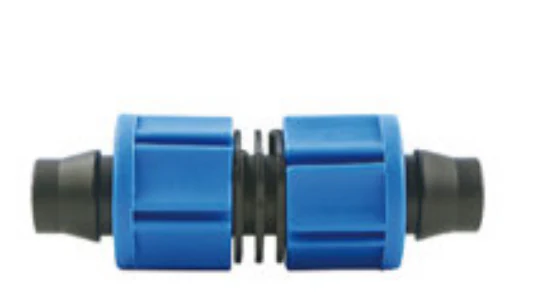
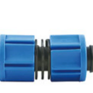
Coupling with catalogue-backed technical fields clearly documented. Compare the exact record, variant and project requirements before a technical enquiry.
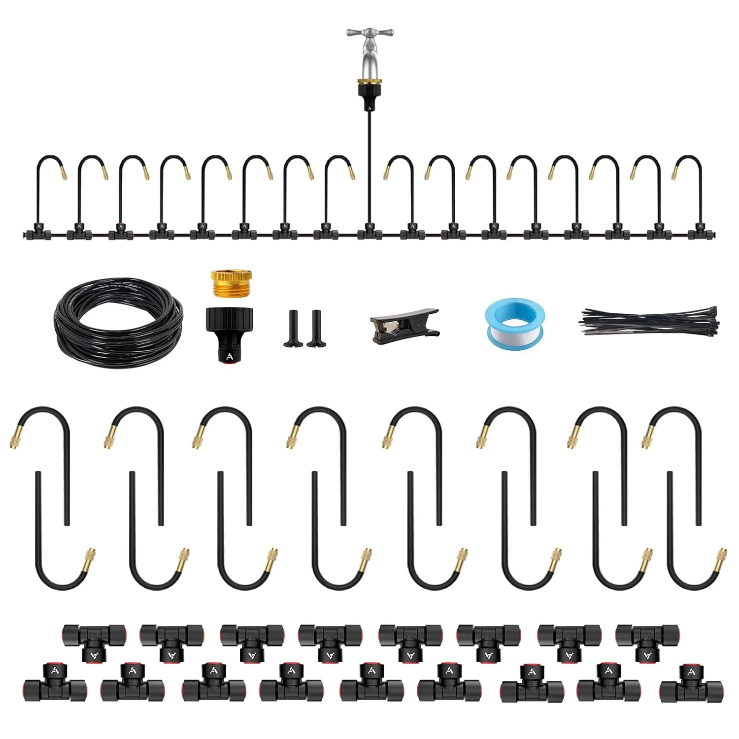
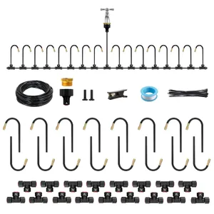
The IrriNex drip irrigation system kit combines 50 ft and 1/4-inch for greenhouses. Review listed components and connection details before ordering.
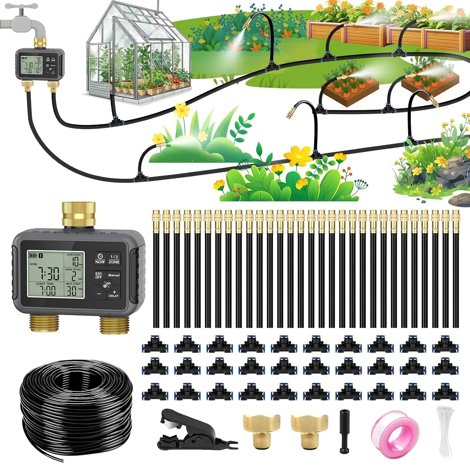
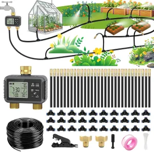
The IrriNex drip irrigation system kit combines 120 ft for raised beds and vegetable gardens. Review the listed components, connection format and purchase configuration before ordering.
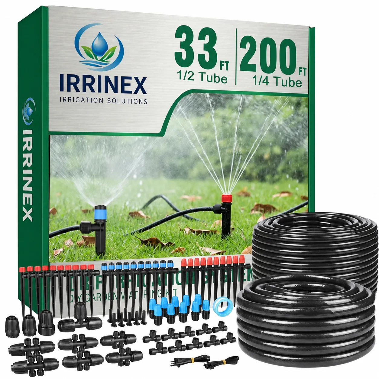
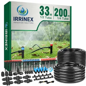
The IrriNex drip irrigation system kit combines 233 ft and 33 ft for raised beds and greenhouses. Review the listed components, connection format and purchase configuration before ordering.