Technical2026-10-26
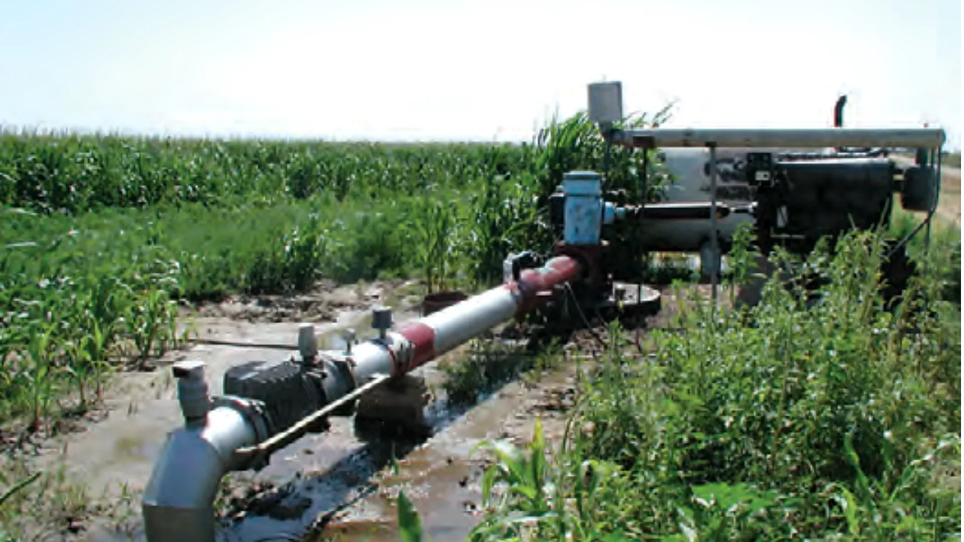
An irrigation pump energy audit should report the electricity used for each cubic metre actually delivered during the same test window. Read the energy meter and the irrigation water totalizer at the start and end of a stable run, subtract both pairs of readings, then divide the measured kilowatt-hours by the measured cubic metres. The result, kWh/m³, is a field performance indicator for that pump, water source, hydraulic duty and test boundary.
The ratio becomes misleading when energy and water cover different times, when another load shares the electrical meter, or when two tests require different lift and pressure. This guide sets a repeatable boundary, gives a worked calculation, and shows how to compare like duties without inventing a universal efficiency threshold.
The indicator answers a practical accounting question: how much purchased electrical energy crossed the selected boundary while one cubic metre of irrigation water crossed the matching water boundary? A lower value can mean better performance, but it can also mean that the second test lifted water through less head. The number is therefore a trend and comparison tool, not a stand-alone verdict on pump condition.
Benchmarking energy consumption across off-grid agricultural blocks involves testing the electrical efficiency of solar DC brushless centrifugal pumps delivering pressurized water to remote field emitters.
Use kWh/m³ to compare the same pump over time, rank parallel pumps serving an equivalent duty, verify a change after maintenance, or convert an energy tariff into a pumping cost per delivered volume. Keep flow, pressure, pumping water level, zone configuration and filter condition beside the ratio. These measurements explain why it moved.
Draw two boundaries on a simple pump-station sketch. The electrical boundary must include the equipment whose consumption will be reported. The water boundary must include the flow represented by the totalizer. If the energy meter includes a booster, filter-backwash pump or building load that the water meter does not represent, the ratio is not pump-specific. Either isolate those loads or label the result as a station-level indicator.
State whether the test begins at the utility meter, a dedicated motor meter, or a temporary power analyzer. State whether water is measured at the well discharge, after filtration, or at the field inlet. The start and end timestamps must match. The irrigation flow-meter pulse guide explains how to verify units, multipliers and totalizer increments before relying on a remote count.
| Field | Why it matters | Recording rule |
|---|---|---|
| Energy-meter ID and boundary | Shows which loads are included | List every motor or auxiliary load downstream of the meter |
| Water-meter ID and boundary | Links energy to the matching delivered volume | Record location, unit and multiplier |
| Start and end readings | Creates auditable differences | Use cumulative readings, not a copied dashboard average |
| Start and end timestamps | Proves synchronized sampling | Use one clock and document time zone |
| Flow and discharge pressure | Defines the operating duty | Record stabilized values and instrument locations |
| Pumping water level or suction condition | Captures changing lift | Measure by an appropriate safe method |
| Valve, zone and speed state | Prevents unlike configurations being mixed | Use a fixed configuration code |
| Filter and backwash state | Separates restriction and auxiliary consumption | Record differential pressure and timed events |
Choose a normal irrigation job with a defined zone set, target pressure and pump speed. Avoid startup, shutdown and deliberate flushing unless the objective is to audit the entire cycle. If the system serves changing zone demands, use the pump and system curve guide to identify which duties are physically comparable.
Minimizing head loss across station control manifolds reduces total kWh demand, prompting audit teams to verify that low-friction solenoid control valves exhibit internal pressure drops below 0.25 bar at design flow.
Confirm that the electrical display is cumulative kWh and that the water display is cumulative m³. If the water meter uses litres, gallons, pulses or a displayed multiplier, convert only after recording the original values. Note who owns sealed revenue metering and do not open energized panels. Electrical measurements beyond a normal display should be made by a qualified person using suitable equipment and procedures.
Run the intended zone until pipe filling, air release, valve travel and pressure-regulator movement have settled. Record flow, discharge pressure, filter differential pressure, speed and source level. Stability should be judged from observations, not from an arbitrary delay copied from another farm.
Photograph or transcribe the energy and water totalizers and record the time. If one person cannot see both instruments, use synchronized clocks and a documented communication sequence. The timing error should be small relative to the test length and stated meter resolution.
Do not add a zone, change a pressure setpoint, run a backwash cycle or energize another downstream load without recording the event. If a necessary event changes the boundary, end the interval and start a new one. A long mixed interval is not automatically better than a shorter clean interval.
Use the same method and instrument displays as at the start. Verify that neither meter rolled over and that remote data contain no gaps. Record ending pressure, flow, water level and speed so the operator can see whether the duty drifted during the run.
Subtract the start from the end for energy and volume. Calculate kWh/m³, average kW and average m³/h. Retain the photographs or raw exports, configuration code and observations. A spreadsheet result without its two meter differences cannot be independently checked.
Use cumulative differences because they integrate the whole test window:
Energy used (kWh) = ending kWh - starting kWh
Volume delivered (m³) = ending m³ - starting m³
Specific energy (kWh/m³) = energy used ÷ volume delivered
As a cross-check, calculate average kW = kWh ÷ hours and average flow = m³ ÷ hours. Dividing average kW by average m³/h should return the same kWh/m³, apart from rounding. If it does not, revisit units, timestamps and meter scaling.
Do not substitute motor nameplate kW for measured energy. A nameplate describes rated equipment, while actual input depends on load, efficiency, voltage, power factor and operating point. The irrigation pump sizing guide remains useful for the design duty, but an energy audit must measure the installed system.
Suppose a dedicated electricity meter reads 12,840.6 kWh at the start and 12,924.6 kWh two hours later. The matching water totalizer moves from 46,520 m³ to 46,940 m³. During the interval, the same irrigation block remains open and pressure, flow and pumping water level stay within the accepted test envelope.
| Quantity | Calculation | Result |
|---|---|---|
| Electricity | 12,924.6 - 12,840.6 | 84.0 kWh |
| Delivered water | 46,940 - 46,520 | 420 m³ |
| Specific energy | 84.0 ÷ 420 | 0.200 kWh/m³ |
| Test duration | Ending time - starting time | 2.00 h |
| Average input power | 84.0 ÷ 2.00 | 42.0 kW |
| Average flow | 420 ÷ 2.00 | 210 m³/h |
| Example energy cost | 0.200 × 0.16 currency/kWh | 0.032 currency/m³ |
The tariff is an example only; use the actual energy charge and treat demand charges, time-of-use rates, taxes and fixed fees separately. The calculated 0.200 kWh/m³ belongs to this test boundary and duty. It is not a universal target for irrigation pumps.
Energy per volume must rise when the pump does more hydraulic work, even if equipment efficiency is unchanged. Total dynamic head includes source lift, required outlet pressure, elevation change and losses through pipe, valves and filtration. Compare repeat tests at equivalent flow, pressure, pumping water level and configuration, or explicitly normalize the analysis with a complete head measurement.
For water, the ideal hydraulic energy per cubic metre can be written as 0.002725 × head in metres kWh/m³. At 40 m of head, the ideal water-side energy is about 0.109 kWh/m³. If measured input is 0.200 kWh/m³ at that fully measured head, the illustrative overall efficiency is approximately 0.109 ÷ 0.200 = 54.5%. This example demonstrates the relationship; it does not set an acceptance threshold.
A drop in well water level increases lift. A loaded filter increases loss. A higher pressure setpoint adds work. Before attributing a change to the pump, inspect the hydraulic budget and the operating point. Where speed changes with zone demand, consult the multi-pump station sequencing guide for the controls that can change which equipment is inside the test.
Treat the ratio as the first line of a diagnosis. A higher value can result from more head, lower pump or motor efficiency, reduced flow, an electrical problem, a water-meter error, or an added load inside the energy boundary. A lower value can be real improvement, but it can also follow lower pressure, a shallower pumping water level, an omitted electrical load or overstated water volume.
| Observed pattern | Possible explanation | First verification |
|---|---|---|
| kWh/m³ up; head up | Deeper water level, higher setpoint or added friction | Recalculate total dynamic head |
| kWh/m³ up; head similar; flow down | Wear, blockage, recirculation or operating-point shift | Verify meter and compare pump curve |
| kWh/m³ up after filter loading | Added differential pressure | Record clean and loaded filter readings |
| kWh/m³ jumps with no hydraulic change | Auxiliary load or electrical-meter boundary changed | Inventory downstream loads and meter IDs |
| kWh/m³ falls with pressure | Less delivered duty rather than an efficiency gain | Check pressure at the required service point |
| Ratio erratic between identical runs | Short sample, clock mismatch or coarse meter resolution | Lengthen a stable test and synchronize readings |
| Off-cycle energy or water movement | Standby load, valve leakage or unintended flow | Separate closed-valve and energized-state checks |
The USDA Natural Resources Conservation Service describes a pumping-plant evaluation that gathers flow, pressure or head, energy use and site data under a defined operating condition. Its Irrigation Pumping Plants engineering handbook also stresses safe, qualified measurement around operating electrical and mechanical equipment.
Water-side errors include a partly full pipe, poor meter placement, an incorrect pulse factor, an unrecorded bypass or a totalizer in the wrong unit. Energy-side errors include using kW instead of kWh, including unrelated loads, reading different tariff registers, or estimating energy from horsepower. Boundary errors occur when the water and energy intervals do not represent the same operation.
Check each side independently. Compare remote water totals with the local register. Compare interval energy with average kW multiplied by time. Reconcile runtime against controller logs. The pump and valve interlock guide helps identify energized periods when no intended delivery path is open.
Commission a baseline only after the instruments and hydraulic condition have been verified. Store several healthy runs rather than one favorable number. Group results by source level, pressure setpoint, active zone, speed band and filter state. Use a control chart or a simple median and observed range, but keep the raw values and measurement uncertainty.
Do not copy a universal percentage trigger. Set investigation limits from meter resolution, healthy repeatability, the cost of excess energy and the operational consequences of missed faults. A sustained change under equivalent duty is more persuasive than one isolated reading. After repair, repeat the same test to prove whether the intervention improved energy per delivered volume.
$$SEC (\text{kWh}/\text{m}^3) = \frac{P_{\text{electric}} (\text{kW})}{Q (\text{m}^3/\text{h})}$$ For example, a pump drawing $45\text{ kW}$ while delivering $150\text{ m}^3/\text{h}$ has an $SEC = 45 / 150 = 0.30\text{ kWh}/\text{m}^3$.
$$WTE = \frac{P_{\text{water}}}{P_{\text{electric}}} = \frac{Q (\text{m}^3/\text{s}) \times H (\text{m}) \times 9.81}{P_{\text{electric}} (\text{kW})}$$ Commercial Benchmarks: Excellent: $\ge 65\% - 72\%$; Acceptable: $55\% - 64\%$; Poor / Needs Immediate Overhaul: $< 50\%$.
Internal sand erosion: sand particles erode the fine running clearances between the impeller wear rings and casing from 0.3mm out to 2.0mm. Water recirculates continuously inside the casing, wasting massive amounts of electric power.
Because inductive motors have a power factor ($PF$) and phase angle. True power must be measured using a true-RMS power quality meter: $$P (\text{kW}) = \frac{\sqrt{3} \times V_{\text{line}} \times I_{\text{line}} \times PF}{1000}$$
Products relevant to this irrigation guide.

IRRINEX compression pipe fitting. Diameter: 16/20/25/32mm; Diameter: 20mm; Size: 16/20/25/32mm. A compression fitting joins a matched pipe to the selected connection. Check each pipe and thread dimension for the exact fitting configuration.
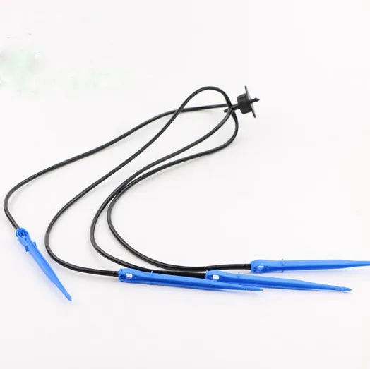
IRRINEX arrow dripper. Flow rate: 4*1.5. An arrow dripper places a drip outlet at a planting point. Select the branch and tubing arrangement from the configuration actually documented for this listing.
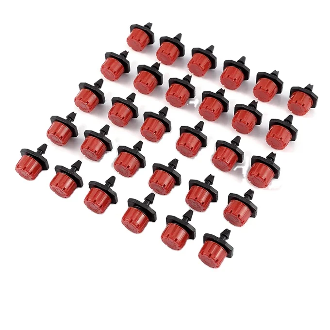
IRRINEX adjustable irrigation dripper. Flow Rate: 0-70L/h. An adjustable dripper is selected for a point-watering arrangement. The chosen setting should be checked under the site's actual operating conditions.

IRRINEX impact sprinkler. Size: 1" Male Thread; Working Pressure: 2.0-5.0bar; Spraying Radius: 20-25m. An impact sprinkler distributes water from a selected sprinkler position. Choose the exact connection and nozzle configuration using the recorded pressure and discharge information.